Crime Analysis

For the first main topic in Applications in GIS, we covered crime analysis, which I found interesting for a few reasons. First, I have not covered the use or application of GIS in the crime field in the certificate program courses up until now, so I enjoyed learning how the technologies can be applied to this type of phenomena.  Another reason of interest is that part of my academic background is in the field of sociology. The first sociology department founded in the U.S.A. was at the University of Chicago (in 1892) and some of the earliest research conducted by pioneering sociologists in this organization focused on the relationship between demography, geography, and crime, such as the work of Shaw and Mckay.  While sociologists use some of the same analytical and statistical methods as geographers/GIS professionals in the analysis of crime (rates, incidences, etc.), there are some fundamental differences!  I cannot recall covering kernel density estimation or Moran I’s in my sociology of crime graduate seminar. 

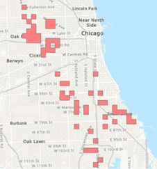
For the module's assignment, I created maps from crime data, including homicides in Chicago in 2017 and 2018. The three images below shows maps of homicides in 2017. These include: a grid overlay thematic map showing areas with the top 20% of homicides in Chicago in 2017, a kernel density map showing areas with homicides 3 times the mean average, and a local Moran's I map showing areas aggregated by meaningful boundaries:

Grid overlay showing areas with the top 20% of homicides

 
Kernel density showing areas with a homicide rate triple the city's average

 

 
Local Moran's I showing areas of high crime bounded by meaningful boundaries

As part of our assignment, we were tasked with providing a hypothetical policy recommendation to a police administrator that would best help them determine which map would be the most useful to them in terms of allocating limited policing resources within the city. I recommend the Kernel Density map, because they can focus resources on areas with the highest density of homicides with a prediction rate that is almost the best. With Kernel Density we are examining areas that have triple the mean homicide rate whereas with the grid overlay we are just looking at areas with the top 20%.  Local Moran I’s does cluster high values with aggregated boundaries, but the area appears broad on the map and could constrain police time and resource availability. 

Overall, I enjoyed completing this assignment very much because it provided me with a new way to examine spatial patterns of crime in a more comprehensive and productive way that through sociology.  It has also provided me with some suggestions for activities that I can employ in some of my own classes.