Jason's GeoJourney

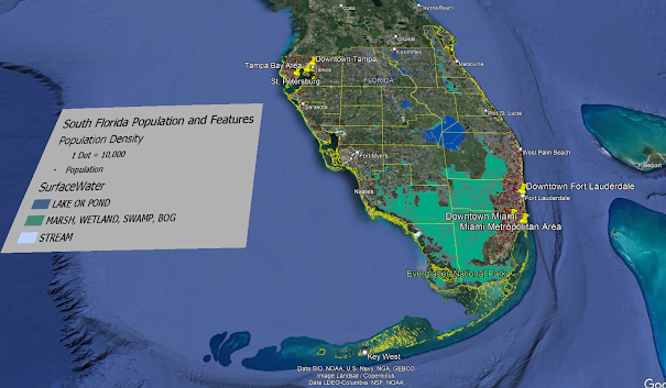
This week in Computer Cartography, I completed the last course module which involved the creation of a Google Earth map showing the locations of 23 south Florida counties, their population densities, and surrounding water features.  To do this, I converted dot density and surface water layers in ArcGIS to KML (KMZ files) then imported into Google Earth.  Previously, I adjusted the symbology for three distinct water features in the surface water layer to correspond to the provided legend.  After the KMZ files were opened in Google Earth, I added the legend, and then adjusted the borders for the 23 counties in yellow.  I ended with preparing a recorded tour with narration showing the locations of six areas:  the Miami metropolitan area, Downtown Miami, Downtown Fort Lauderdale, the Tampa Bay area, St. Petersburg, and Downtown Tampa.  To do this, I created place marks for each of these areas, then used the Record a Tour feature. In my tour, I gave general reference to significant environm

This week in Computer Cartography we learned about isarithmic mapping. For our lab activity, our primary task was to create a map illustrating a nnual precipitation data for the State of Washington from 1981 to 2010 that was derived and interpolated by using PRISM (Parameter-elevation Relationships on Independent Slopes Model) which accounts for how elevation influences climate patterns, as in this case precipitation. By using point data from a 30-year climatological average with an underlying digital elevation model (DEM), estimates of precipitation are shown in a continuous tone where hypsometric tinting was applied to highlight patterns of elevation with matching contours.   I appreciate the opportunity that this week's module has provided to me in learning about this type of mapping.  I could envision application of isarithmic maps in some of my own research, such as in conveying deeper historical data on climate or illuminating the dynamics of other variables such as human tra

For this week’s module in Computer Cartography, I created a map that displays the rate of wine consumption in relation population density for 34 European countries.   For the primary map, I used custom graduated symbols by creating a five-tier wine bottle marker scheme, to show different levels of wine consumption per capita for each country (litter/person).   I did this by downloading a creative commons/free .jpg of a wine bottle, editing it to show a green base (for the bottle/container) and then creating five different versions with purple fill to show different levels of consumption (the most filled with purple, the highest level).   I then converted these to individual .svg files to import into ArcGIS.   Further, I did use some proportional scaling to size each one different (the larger the bottle, the higher the wine consumption) to better convey the variation along with the level of purple fill. To show population density of the associated European countries, I used a light

This week in Computer Cartography we covered data classification where we were directed to produce maps showing the distribution of senior citizens (individuals above the age of 65) in Miami-Dade County in tract data from the U.S. Census of 2010.   For the main objective, students were tasked to use and assess four different methods of data classification in this pursuit:   equal interval, quantile, natural breaks, and standard deviation.   Further, we needed to use two different variables from the census data:   the percentage of individuals above 65 and the number of individuals (normalized by square mile) above 65.   A total of eight maps were produced with four comprising a composite related to each of the two different age variables.   In addition, I selected one of the eight that I felt best conveys the distribution of seniors in Miami-Dade County.I used a green continuous choropleth scheme for all of the maps except for the ones classed on standard deviation. The only adjustment

This week’s module in GIS 5007 covered cartographic design principles where we were directed to produce a map of public schools in Ward 7 of Washington, D.C. One of the main objectives of the assignment was to employ Gestalt principles of perceptual organization related to cartographic design. By employing visual hierarchy, I made sure to give the thematic symbols and type labels the highest priority.   I clipped the Ward 7 schools from the DC schools layer, and then assigned unique symbological values to elementary, middle, and high schools by using three distinct school house icons from small to large respectively.   For the three school types, I used red-orange fonts then set the size for each at three different levels (Tuscan red 26 pt for high schools, Flame red 24 pt for middle schools, and Seville orange 22 pt font for elementary schools). Each school was labeled with a number that corresponded with a list place in the top right corner.   Each school was labeled with Tahoma 10