Data Quality: Fundamentals

This week, I completed the first assignment in the Special Topics in GIS (GIS 5935) class.  Here we learned about calculating metrics for spatial data quality in GIS, specifically understanding the difference between assessments of precision and accuracy. According to Boldstad and Manson (2022:610), "accuracy is most reliably determined by a comparison of true values to the values represented in a spatial data set." Precision, in contrast refers to "the consistency of a measurement method" (2022:612). Unlike accuracy, precision does not use a reference value but instead assesses the variance of values in the data set.

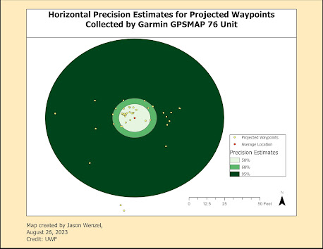
In the first part of the lab, horizontal accuracy was determined from 50 waypoints mapped with a Garmin GPSMAP 76 unit, which according to the manufacturer, this device is "accurate to within 15 meters (49 feet) 95% of the time" where "users will see accuracy within 5 to 10 meters (16 to 33 feet) under normal conditions." For the exercise, I aggravated the 50 waypoints into a new average waypoint spapefile, then projected this and the original waypoints shapefile into the appropriate coordinate system (NAD 1983 UTM Zone 17N). By using the Spatial Join tool, distance from the average waypoint to each location could be determined. Following this, I created three buffers around the average waypoint location that encompassed 50%, 68%, and 95% of horizontal accuracy errors:

The distance between the average location and reference point was 3.5 meters.  This is between the 50% buffer of 3.0 meters and the 68% buffer of 4.2 meters. The results indicate that the GPS unit has an accuracy of 4.2 meters for 68% of points collected. 95% of the errors fell within 15.8 meters, which is slightly higher than Garmin's claim for 95% accuracy within 15 meters. However, given the accuracy of 4.2 meters for 68% (within one standard deviation) this is under the threshold claim of Garmin of 5 to 10 meters of accuracy.

For the second part of the exercise, I used root-mean-square-error (RMSE) and cumulative distribution function (CDF) to determine the distribution of errors in a larger data set. The CDF provides insights into how the probability of a random value accumulates over time, which is different than what the metrics provide about how these errors are distributed within a population.

Here I learned how to extract tabular data from a .dbf in MS Excel and used various formulates to determine the errors:

Data Quality Assessment	50%	68%	95%
Horizontal Accuracy	3.02	6	15.8
Horizontal Precision	3	4	17
Vertical Accuracy	4.2	5.85	18
Vertical Precision	4.2	5.85	18.3

Overall, I found this week's topic and lab to be interesting and helpful in furthering developing my GIS skills.  I have had a limited understanding in assessing data quality up until this module, but I believe this topic is important to GIS analysts given the crucial need to be aware of any errors or biases in the data used.

2022  Boldstad, Paul and Steven Manson
      GIS Fundamentals:  A First Text on Geographic Information Systems, 7th edition. Minnesota:  Eider
      Press.